add_s = function(x){
  y = c("*and$", "*bel$", "*tel$", "*hel$", "*uod$", "*yod$", "*hod$", "*mod$", "*ent$", "*ert$", "*ept$", "*ult$", "*cid$", "*bid$", "*lid$", "*gid$", "*hid$", "*rid$", "*sid$", "*alf$", "*oll$", "*ist$")
  s = sapply(y, function(i){grep(i, x)})
  if(sum(unlist(s))>0){
    x = paste0(x, "s")
  }
  x
}
match_tax = function(i, x){
  x <- x[agrep(i, x$SSL_classification_name, ignore.case=TRUE, max.distance=0.02),]
  if(nrow(x)>0){
    x$taxsubgrp <- i
    return(x)
  }
}USDA Soil Taxonomy training points
USDA soil taxonomy
USDA Soil Taxonomy is among the most described soil classification system in the world with many documents available in open domain and maintained (curtesy of USDA and USGS). The current edition of the Soil Taxonomy is 13 and has 6 levels: Order, Suborder, Great Group, Subgroup, Family, and Series. In this notebook we explain how to produce consistent global analysis-ready point data set with soil taxonomy subgroup labels. Note: this code is continuously being updated. If you have more data you would like to share and add to this list, please contact us.
First we will define two functions to help us clean-up and bind soil type labels. The first function is used to add “s” at the end of the soil label (often ommitted), the second function is used to do a fuzzy search to find is some label appears in complex text:
This is an example of addition of “s” at the end of soil type:
sapply(c("typic argiustoll", "typic argiustolls", "typic haploperox", "aquollic hapludalf", "aquollic hapludalfs"), add_s) typic argiustoll typic argiustolls typic haploperox
"typic argiustolls" "typic argiustolls" "typic haploperox"
aquollic hapludalf aquollic hapludalfs
"aquollic hapludalfs" "aquollic hapludalfs" This is an example of fuzzy search of some target term:
x = data.frame(SSL_classification_name=c("pachic argiustolls", "typic argiustoll",
           "argiustolls", "Typic Argiustolls", "typic Argiustols"), row.no=1:5)
match_tax(i="typic argiustolls", x)
SSL_classification_name row.no taxsubgrp
2 typic argiustoll 2 typic argiustolls
4 Typic Argiustolls 4 typic argiustolls
5 typic Argiustols 5 typic argiustollsAs demonstrated, this will take care of typos and any capital letter issues.
Note that many soil data bases do not have standardized way the soil types are entered and hence some clean-up and sorting is often required. In the case of the National Cooperative Soil Survey Characterization Database, soil types are entered via several columns, which can also be split if needed:
 $ SSL_name                 : chr  NA NA "Cathay" NA ...
 $ SSL_class_type           : chr  NA NA "series" NA ...
 $ SSL_classdate            : chr  NA NA "1991/10/03 00:00:00+00" NA ...
 $ SSL_classification_name  : chr  NA NA "Fine-loamy, mixed, frigid Udic Argiboroll" NA ...
 $ SSL_taxorder             : chr  NA NA "mollisols" NA ...
 $ SSL_taxsuborder          : chr  NA NA "borolls" NA ...
 $ SSL_taxgrtgroup          : chr  NA NA "argiborolls" NA ...
 $ SSL_taxsubgrp            : chr  NA NA "udic argiborolls" NA ...
 $ SSL_taxpartsize          : chr  NA NA "fine-loamy" NA ...
 $ SSL_taxpartsizemod       : chr  NA NA NA NA ...
 $ SSL_taxceactcl           : chr  NA NA NA NA ...
 $ SSL_taxreaction          : chr  NA NA NA NA ...
 $ SSL_taxtempcl            : chr  NA NA "frigid" NA ...
 $ SSL_taxmoistscl          : chr  NA NA NA NA ...
 $ SSL_taxtempregime        : chr  NA NA "frigid" NA ...
 $ SSL_taxminalogy          : chr  NA NA "mixed" NA ...
 $ SSL_taxother             : chr  NA NA NA NA ...
 $ SSL_osdtypelocflag       : int  NA NA NA NA NA NA NA NA NA NA ...
The table TAXOUSDA_GreatGroups.csv contains all combinations of USDA great-groups
sel.tax.vars = c("site_key", "olc_id", "year", "source_db", "longitude_decimal_degrees", "latitude_decimal_degrees", "taxsubgrp")
usda_tax = read.csv("./correlation/TAXOUSDA_GreatGroups.csv")
head(usda_tax)
Great_Group Suborder Order TAX Organic_soils
1 Albaqualfs Aqualfs Alfisols Alfisols_Aqualfs_Albaqualfs 0
2 Cryaqualfs Aqualfs Alfisols Alfisols_Aqualfs_Cryaqualfs 0
3 Duraqualfs Aqualfs Alfisols Alfisols_Aqualfs_Duraqualfs 0
4 Endoaqualfs Aqualfs Alfisols Alfisols_Aqualfs_Endoaqualfs 0
5 Epiaqualfs Aqualfs Alfisols Alfisols_Aqualfs_Epiaqualfs 0
6 Fragiaqualfs Aqualfs Alfisols Alfisols_Aqualfs_Fragiaqualfs 0Preparation of the standard finit legend
In this section we show how to prepare a fixed legend for the purpose of spatial analysis, and which we think represent all world soils. We focus on the “subgroup” e.g. “aeric fluvaquents” (order: Entisols, suborder: Aquents, great group: Fluvaquents), which is an Entisols on floodplains with aquic moisture regimes that are not so wet. They are better aerated in the “upper” part of the soil profile.
To create a representative legend, we will use the highest quality data with soil types quality controlled and described in metadata:
- National Soil Information System (NASIS) profiles and semi-profiles,
- National Cooperative Soil Survey Characterization Database,
- WoSIS soil profiles and samples,
We import the 3 data sets in R:
if(!exists("tax_nasis")){
  ## USDA legacy points ----
  tax_nasis = readRDS.gz(paste0(drv, "USA/NASIS_PNTS/nasis_tax_sites.rds"))
  tax_nasis = plyr::rename(tax_nasis, c("x_std"="longitude_decimal_degrees", "y_std"="latitude_decimal_degrees", "obsdate"="site_obsdate"))
  tax_nasis$source_db = "USDA_NASIS"
  tax_nasis$site_key = paste0("NASIS.", tax_nasis$peiid)
  tax_nasis$olc_id = olctools::encode_olc(tax_nasis$latitude_decimal_degrees, tax_nasis$longitude_decimal_degrees, 11)
  #summary(as.factor(tax_nasis$taxsubgrp))
  tax_nasis$year = as.numeric(substr(tax_nasis$site_obsdate, 1, 4))
  tax_nasis = tax_nasis[,sel.tax.vars]
  tax_nasis = tax_nasis[!is.na(tax_nasis$taxsubgrp) & !is.na(tax_nasis$longitude_decimal_degrees),]
}
str(tax_nasis)
'data.frame': 314560 obs. of 7 variables:
$ site_key : chr "NASIS.115624" "NASIS.115623" "NASIS.9914" "NASIS.9948" ...
$ olc_id : chr "85V4PQC2+G3V" "85V4QW49+6PQ" "84PRGC6X+2JP" "84PRCCV7+MXV" ...
$ year : num 2000 2000 2000 2000 2000 2000 2000 2000 2000 2000 ...
$ source_db : chr "USDA_NASIS" "USDA_NASIS" "USDA_NASIS" "USDA_NASIS" ...
$ longitude_decimal_degrees: num -117 -117 -124 -124 -117 ...
$ latitude_decimal_degrees : num 47.7 47.8 44.5 44.4 47.2 ...
$ taxsubgrp : chr "xeric argialbolls" "aquandic humaquepts" "pachic fulvicryands" "lithic hapludands" ...if(!exists("ncss.site")){
ncss.site <- read.table(paste0(drv, "INT/USDA_NCSS/ncss_labdata_locations.csv.gz"), fill = TRUE, header = TRUE, sep=",")
#str(ncss.site)
ncss.site = plyr::rename(ncss.site, c("corr_taxsubgrp"="taxsubgrp"))
ncss.site$source_db = "USDA_NCSS"
ncss.site$year = as.numeric(substr(ncss.site$site_obsdate, 1, 4))
ncss.site$olc_id = olctools::encode_olc(ncss.site$latitude_decimal_degrees, ncss.site$longitude_decimal_degrees, 11)
ncss.site = ncss.site[,sel.tax.vars]
ncss.site = ncss.site[!is.na(ncss.site$taxsubgrp) & !is.na(ncss.site$longitude_decimal_degrees),]
#summary(as.factor(ncss.site$taxsubgrp))
}
dim(ncss.site)[1] 33235 7if(!exists("tax_wosis")){
tax_wosis = readr::read_tsv(gzfile(paste0(drv, 'INT/WoSIS/WoSIS_2023_December/wosis_202312_profiles.tsv.gz')), col_types='icciccddcccccciccccicccci')
tax_wosis = plyr::rename(tax_wosis, c("longitude"="longitude_decimal_degrees", "latitude"="latitude_decimal_degrees", "dataset_code"="source_db"))
tax_wosis = tax_wosis[!is.na(tax_wosis$usda_great_group),]
tax_wosis$taxsubgrp = tolower(paste(tax_wosis$usda_subgroup, tax_wosis$usda_great_group))
tax_wosis$site_key = paste0("WOSIS.", tax_wosis$site_id)
tax_wosis$year = as.numeric(substr(tax_wosis$usda_publication_year, 1, 4))
tax_wosis$olc_id = olctools::encode_olc(tax_wosis$latitude_decimal_degrees, tax_wosis$longitude_decimal_degrees, 11)
tax_wosis = tax_wosis[,sel.tax.vars]
tax_wosis = tax_wosis[!is.na(tax_wosis$taxsubgrp) & !is.na(tax_wosis$longitude_decimal_degrees),]
#summary(as.factor(tax_wosis$taxsubgrp))
}
dim(tax_wosis)[1] 30998 7UK LandIS augers and profiles also contain a lot of ground data with soil types:
if(!exists("tax_landis")){
  tax_landis = read.csv(paste0(drv, 'UK/landis/AUGERsite_3528240497585825957.csv'), stringsAsFactors = FALSE)
  #head(sort(table(as.factor(tax_landis$SERIES_NAME)), decreasing = TRUE), 10)
  #   UNKNOWN BRICKFIELD   HIGHWEEK    ANDOVER       WICK    WHIMPLE      MANOD
  #   15591       3409       2422       2269       2264       2190       2134
  # CLIFTON    EVESHAM    NEWPORT
  #    1996       1961       1869
  tax_landis$SERIES_NAME = ifelse(tax_landis$SERIES_NAME=="HIGHWEEK", "DENBIGH", tax_landis$SERIES_NAME)
  ## convert to lon-lat coordinates
  landis.coords = as.data.frame(geom(terra::project(terra::vect(tax_landis[,c("EASTING","NORTHING")], geom=c("EASTING","NORTHING"), crs="EPSG:27700"), "EPSG:4326"))[,c("x","y")])
  tax_landis$longitude_decimal_degrees = landis.coords$x
  tax_landis$latitude_decimal_degrees = landis.coords$y
  cor.landis = read.csv('correlation/UK_landis_correlation.csv')
  tax_landis$taxsubgrp = tolower(plyr::join(tax_landis, cor.landis, match = "first")$USDA_correlation)
  tax_landis$source_db = "UK LandIS"
  tax_landis$site_key = paste0("LandIS.", tax_landis$AUGERID)
  tax_landis$site_obsdate = format(as.Date(tax_landis$SURVEY_DATE, format="%m/%d/%Y"), "%Y-%m-%d")
  tax_landis$year = as.numeric(substr(tax_landis$site_obsdate, 1, 4))
  tax_landis$olc_id = olctools::encode_olc(tax_landis$latitude_decimal_degrees, tax_landis$longitude_decimal_degrees, 11)
  tax_landis = tax_landis[,sel.tax.vars]
  tax_landis = tax_landis[!is.na(tax_landis$taxsubgrp) & !is.na(tax_landis$longitude_decimal_degrees),]
  #summary(as.factor(tax_landis$taxsubgrp))
}
Joining by: SERIES_NAMEdim(tax_landis)[1] 104704 7## [1] 104704 7Next, we can bind the 3 data sets to produce 1 consistent legend with finite number of classes and names strictly standardized. We also add “s” to fix typos etc.
if(!exists("tax_all")){
  tax_all = do.call(rbind, list(tax_nasis, tax_wosis, ncss.site, tax_landis))
  #str(tax_all)
  ## 483497 obs. of  7 variables
  ## add missing "s"
  #tax_all$taxsubgrp = sapply(tax_all$taxsubgrp, add_s)
  tax_all$taxsubgrp = unlist(parallel::mclapply(tax_all$taxsubgrp, add_s, mc.cores = 32))
}
#summary(as.factor(tax_all$taxsubgrp[grep("boralf", tax_all$taxsubgrp)]))
summary(as.factor(tax_all$taxsubgrp))
typic epiaquepts typic dystrudepts
26192 17638
aquic hapludalfs typic hapludalfs
14388 12622
typic eutrudepts typic fluvaquents
9007 7707
typic hapludults typic argiustolls
6832 6467
typic haploxererts typic haplorthods
6463 5873
typic udipsamments pachic argiustolls
4912 4611
typic argiudolls mollic hapludalfs
4561 4516
typic paleudalfs aridic argiustolls
4481 4131
typic paleudults typic endoaquolls
4124 3855
aridic haplustalfs typic haplustolls
3682 3590
aridic calciustepts oxyaquic hapludalfs
3479 3389
ustic haplocalcids typic haplustalfs
2979 2832
ultic hapludalfs typic argiaquolls
2738 2636
lithic haplustolls fluvaquentic eutrudepts
2633 2615
typic haplustepts typic hapludolls
2560 2524
aridic haplustepts histic humaquepts
2521 2295
aridic calciustolls ustic haplocambids
2258 2256
typic torriorthents aeric epiaqualfs
2162 2109
ustic calciargids aquic eutrudepts
1991 1969
typic torripsamments lithic udorthents
1960 1949
cumulic hapludolls cumulic haplustolls
1934 1918
ustic haplargids udic argiustolls
1836 1815
aridic paleustolls aquic argiudolls
1810 1798
ustic torriorthents aridic haplustolls
1738 1736
lithic ustic torriorthents typic haplocalcids
1697 1662
pachic haplustolls typic udorthents
1623 1571
aquic hapludults andic haplocryods
1563 1547
ultic haploxeralfs calcidic argiustolls
1543 1541
oxyaquic argiudolls typic fragiudults
1539 1506
typic sphagnofibrists typic psammaquents
1493 1488
aridic paleustalfs typic haplosaprists
1446 1443
cumulic endoaquolls typic dystrocryepts
1414 1394
typic haplocryepts typic eutrocryepts
1375 1358
ustic torripsamments aridic ustorthents
1348 1342
aquertic argiudolls udic haplusterts
1323 1312
typic cryorthents fluvaquentic endoaquepts
1305 1298
ustic argicryolls typic argixerolls
1290 1285
typic epiaqualfs typic kanhapludults
1240 1222
terric haplosaprists aquic dystrudepts
1211 1209
typic calciustolls lithic argixerolls
1207 1204
typic udifluvents typic ustorthents
1204 1195
dystric eutrudepts oxyaquic fragiudalfs
1186 1184
fluvaquentic endoaquolls typic histoturbels
1163 1162
aquic udipsamments aquic hapludolls
1151 1139
pachic argicryolls typic endoaqualfs
1133 1132
calcidic haplustalfs petrocalcic calciustolls
1102 1083
typic haplocambids typic haplargids
1081 1052
calcic petrocalcids lithic hapludolls
1027 1009
xeric haplargids lithic torriorthents
965 957
typic glossaqualfs (Other)
957 197524 This shows which are the world’s most frequent subgroup classes. Next we can complete the final legend. For practical purposes, we limit to classes that have at least 30 observations, which gives a total of 818 classes.
#write.csv(ext.l, "tax_extensions_summary.csv")
tax.sm = summary(as.factor(tax_all$taxsubgrp), maxsum = 820)
tax.s = as.data.frame(tax.sm)
levels = attr(tax.sm, "names")[1:818]
write.csv(tax.s, "correlation/tax_taxsubgrp_summary.csv")
It is important for further spatial analysis that the number of classes is finite and that there are enough points for Machine Learning for example.
Fuzzy search
Next, we would also like to add points from national and regional soil profiles that are not listed above and that could help increase representation of points geographically. For this we use the previously compiled soil data described in the previous sections:
if(!exists("tax_spropsA")){
  tax_sprops0 = as.data.frame( rbind(data.table(readRDS.gz(paste0(drv, "sol_chem.pnts_horizons.rds"))),
                                     data.table(readRDS.gz(paste0(drv, "sol_chem.pnts_horizons_TMP.rds"))), fill=TRUE, ignore.attr=TRUE))
  tax_sprops0 = tax_sprops0[!tax_sprops0$source_db=="USDA_NCSS" & !(tax_sprops0$SSL_classification_name %in% c("", "NA / NA", "#N/A / #N/A", " / ")),]
  tax_sprops0$year = substr(tax_sprops0$site_obsdate, 1, 4)
  tax_sprops0 = tax_sprops0[!duplicated(tax_sprops0$olc_id),]
  tax_sprops0$SSL_classification_name = tolower(tax_sprops0$SSL_classification_name)
  tax_sprops0 = tax_sprops0[!is.na(tax_sprops0$SSL_classification_name),]
  dim(tax_sprops0)
  ## 41067    46
  #summary(as.factor(tax_sprops0$source_db))
  #str(tax_sprops0$SSL_classification_name)
  tax_c1 = sapply(tax_sprops0$SSL_classification_name, function(i){strsplit(i, " / ")[[1]][1]})
  tax_c2 = sapply(tax_sprops0$SSL_classification_name, function(i){strsplit(i, " / ")[[1]][2]})
  sel.tax.vars0 = c("site_key", "olc_id", "year", "source_db", "longitude_decimal_degrees", "latitude_decimal_degrees")
  tax_spropsA = rbind(cbind(tax_sprops0[,sel.tax.vars0], data.frame(SSL_classification_name=tax_c1)),
                      cbind(tax_sprops0[,sel.tax.vars0], data.frame(SSL_classification_name=tax_c2)))
}
str(tax_spropsA)
'data.frame': 98472 obs. of 7 variables:
$ site_key : chr "15" "17" "18" "19" ...
$ olc_id : chr "9F6FRM8J+J62" "9F6CPWCV+9M9" "9F6FP2XH+P9C" "9F6FQ52P+RHW" ...
$ year : chr "2016" "2016" "2015" "2016" ...
$ source_db : chr "BZE_LW" "BZE_LW" "BZE_LW" "BZE_LW" ...
$ longitude_decimal_degrees: num 9.68 8.94 9.03 9.19 9.78 ...
$ latitude_decimal_degrees : num 54.8 54.7 54.7 54.8 54.7 ...
$ SSL_classification_name : chr "typic argiudoll" "aeric tropaquept" "humaquept" "humaquept" ...This gives us additional 100k points with soil classification name. These points need to be cleaned up to match exactly the previously produced legend. Because fuzzy matching can be computational as the algorithm looks for N classes in M rows, we run this matching in parallel:
library(parallel)
tax_spropsA.lst = parallel::mclapply(levels, function(i){match_tax(i, tax_spropsA)}, mc.cores=30)
tax_spropsV = do.call(rbind, tax_spropsA.lst)
## Add missing "S" on the end:
## "paleustollic chromustert" -> "paleustollic chromusterts"
tax_spropsV$taxsubgrp = unlist(parallel::mclapply(tax_spropsV$taxsubgrp, add_s, mc.cores = 30))
str(tax_spropsV)
'data.frame': 33434 obs. of 8 variables:
$ site_key : chr "78" "845" "1472" "10711" ...
$ olc_id : chr "66XR96RR+CFR" "67C29FCP+V2P" "6772QHXM+F2R" "6793JV6J+HH9" ...
$ year : chr "1979" "2010" "2011" "2015" ...
$ source_db : chr "CostaRica" "Ecuador_HESD" "Ecuador_HESD" "Ecuador_HESD" ...
$ longitude_decimal_degrees: num -83.8 -79.5 -79.4 -78.1 -77.4 ...
$ latitude_decimal_degrees : num 9.391 -1.628 -4.201 -2.389 0.121 ...
$ SSL_classification_name : chr "typic epiaquepts" "typic epiaquepts" "typic epiaquepts" "typic epiaquents" ...
$ taxsubgrp : chr "typic epiaquepts" "typic epiaquepts" "typic epiaquepts" "typic epiaquepts" ...this shows that only 34k have an actually matching soil type that we can use.
Final bind
We can finally bind and export the final Analysis-Ready table with training points matching our target legend:
tax_allT = do.call(rbind, list(tax_all, tax_spropsV[,sel.tax.vars]))
str(tax_allT)
'data.frame': 516931 obs. of 7 variables:
$ site_key : chr "NASIS.115624" "NASIS.115623" "NASIS.9914" "NASIS.9948" ...
$ olc_id : chr "85V4PQC2+G3V" "85V4QW49+6PQ" "84PRGC6X+2JP" "84PRCCV7+MXV" ...
$ year : chr "2000" "2000" "2000" "2000" ...
$ source_db : chr "USDA_NASIS" "USDA_NASIS" "USDA_NASIS" "USDA_NASIS" ...
$ longitude_decimal_degrees: num -117 -117 -124 -124 -117 ...
$ latitude_decimal_degrees : num 47.7 47.8 44.5 44.4 47.2 ...
$ taxsubgrp : chr "xeric argialbolls" "aquandic humaquepts" "pachic fulvicryands" "lithic hapludands" ...## 510849 obs. of 7 variables
## we do need duplicates as some translations lead to 2-3 classes
#tax_allT = tax_allT[!duplicated(tax_allT$olc_id),]
## remove all points with exactly the same TAX and olc_id
dup = duplicated(gsub(" ", "_", paste(tax_allT$olc_id, tax_allT$taxsubgrp, sep=" ")))
summary(dup) ## 47811 complete duplicates Mode FALSE TRUE
logical 469120 47811 tax_allT = tax_allT[!dup,]
#summary(as.factor(tax_allT$source_db))
## use only points from the target legend:
tax_allT0 = tax_allT[which(tax_allT$taxsubgrp %in% levels),]
str(tax_allT0)'data.frame': 447124 obs. of 7 variables:
$ site_key : chr "NASIS.275760" "NASIS.9655" "NASIS.9669" "NASIS.9730" ...
$ olc_id : chr "85V565W5+4Q8" "84QRQJP7+9P8" "84QRFHF7+WX6" "84QRMJ24+MPW" ...
$ year : chr "2000" "2000" "2000" "2000" ...
$ source_db : chr "USDA_NASIS" "USDA_NASIS" "USDA_NASIS" "USDA_NASIS" ...
$ longitude_decimal_degrees: num -117 -123 -123 -123 -123 ...
$ latitude_decimal_degrees : num 47.2 45.8 45.5 45.7 44.4 ...
$ taxsubgrp : chr "vitrandic haploxerolls" "dystric eutrudepts" "andic dystrudepts" "humic dystrudepts" ...#write.csv(tax_allT0, gzfile("taxsubgrp_pnts_global_xyt_v20260506.csv.gz"))
#writeVector(vect(tax_allT0, geom=c("longitude_decimal_degrees", "latitude_decimal_degrees"), crs="EPSG:4326"), "/data/wri_soil/taxsubgrp_pnts_global_xyt.gpkg", overwrite=TRUE)Note, we removed some duplicates as many data sets are compilations so some points appear in multiple data sets.
We can plot the density of points in Goode Homolosize Interupted projection so that areas are shown realistically:
g1 = terra::vect(paste0(drv, "tiles_GH_100km_land.gpkg"))
ovt.g1 = terra::extract(g1["ID"], terra::project(terra::vect(tax_allT, geom=c("longitude_decimal_degrees", "latitude_decimal_degrees"), crs="EPSG:4326"), crs(g1)))
g1t.c = summary(as.factor(ovt.g1$ID), maxsum = length(levels(as.factor(ovt.g1$ID))))
g1t.df = data.frame(count=g1t.c, ID=attr(g1t.c, "names"))
g1$count = dplyr::left_join(data.frame(ID=g1$ID), g1t.df)$count
#plot(g1["count"])
writeVector(g1["count"], "/data/dev/tiles_GH_100km_tax.dens.gpkg", overwrite=TRUE)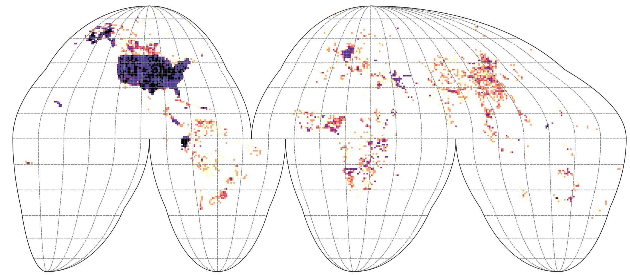
Distribution of training points considering soil orders is:
usda_stats = read.csv("./correlation/TAXSUSDA_stats.csv")
usda_tax$Great_Group = tolower(usda_tax$Great_Group)
usda_stats$Order = dplyr::left_join(usda_stats, usda_tax, by="Great_Group")$Order
o.lst = dplyr::left_join(tax_allT["taxsubgrp"], usda_stats, by=join_by(taxsubgrp==USDA.subgroup))$Order
summary(as.factor(o.lst))
Alfisols Andisols Aridisols Entisols Gelisols Histosols
85420 5569 30805 60400 4559 7875
Inceptisols Mollisols Oxisols Spodosols Ultisols Vertisols
110684 102524 497 14662 20370 16403
NA's
9352 Save temp object:
save.image.pigz(file="soilusda.RData", n.cores = 30)